Reliability Analysis using a Weibull Distribution Model

Modeling Product Lifespan and Assessing Failure Rates with Python.

This Python script is just an example of what you can do with the reliability library we referenced in an earlier post:

Introduction to the reliability Library in Python

It performs a reliability analysis using a two-parameter Weibull distribution model on a simulated set of product lifespan data. The purpose of the analysis is to gain insights into the product's reliability and failure rate over time.

The process begins by generating a synthetic dataset that represents the lifetimes of a batch of products, based on a Weibull distribution which is often used in reliability analysis due to its versatility.

The script then imposes a right-censoring on the data. Right-censoring is a type of data censoring that occurs when the failure time of a unit is not known precisely but is known to exceed a certain value. In this case, any products that did not fail by the 15 time units mark are considered as censored, indicating the test was stopped before they could fail.

Using this censored data, the script fits a two-parameter Weibull distribution. The Weibull distribution is used in reliability studies and survival analysis to represent the time until the occurrence of an event (like a failure), given two parameters - a shape parameter and a scale parameter.

Once the Weibull model is fitted, the script calculates and prints out two key metrics at a specified time point (10 units in this case):

• Reliability (Survival Function): This is the probability that a product survives beyond the specified time.

• Failure Rate (Hazard Function): This is the rate at which failures occur at the specified time.

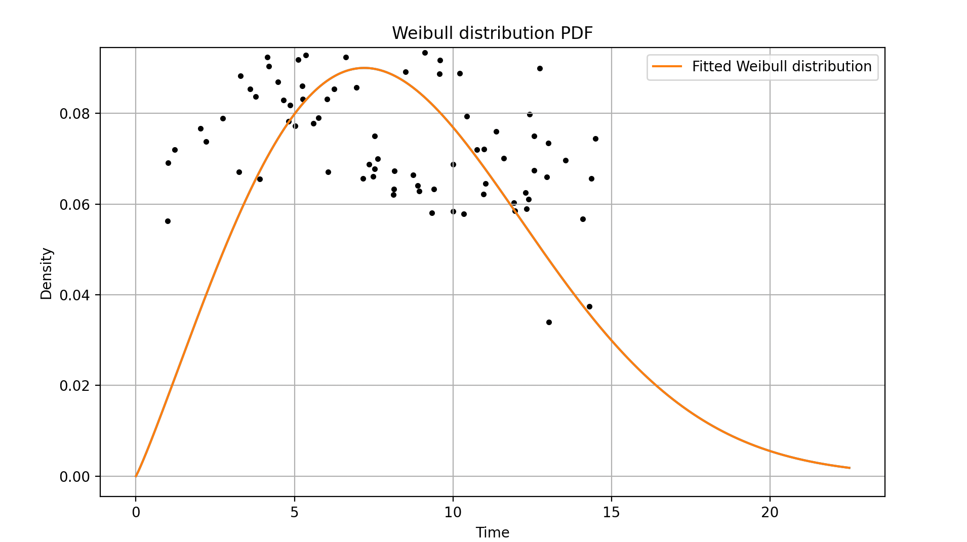
Lastly, the script generates a plot displaying the Probability Density Function (PDF) of the fitted Weibull distribution, providing a visual representation of the failure distribution over time. It also plots the observed failure times and censored times. The generated plot is then saved as a PNG file.

In conclusion, this script is a tool for conducting reliability analysis on product lifespan data, allowing for both statistical and visual assessment of product reliability and failure rate over time.

Step 1: Installing Python

For Windows:

1. Download the latest version of Python 3 from the official site https://www.python.org/downloads/windows/

2. Run the installer file and follow the setup wizard.

3. Ensure the box that says "Add Python 3.x to PATH" is checked. This will add Python to your environment variables, so you can run Python from any command prompt.

4. Click Install, then finish.

For macOS:

1. Download the latest version of Python 3 from the official site https://www.python.org/downloads/mac-osx/

2. Open the downloaded package and follow the setup wizard.

3. After installation, open a terminal window and type python3 to verify the installation.

For Linux (Debian-based distributions like Ubuntu):

1. Open a terminal window.

2. Update package lists for upgrades and new package installations: sudo apt-get update

3. Install Python 3: sudo apt-get install python3

Step 2: Installing pip

pip is the package installer for Python and is normally installed during the Python installation.

Check if pip is already installed:

pip3 --version

If pip is not installed, follow these steps:

For Windows and macOS:

Download the get-pip.py file from https://bootstrap.pypa.io/get-pip.py, then run it with Python:

python3 get-pip.py

For Linux:

In the terminal, run the following command:

sudo apt-get install python3-pip

Step 3: Installing Python Libraries

We will use pip to install the required Python libraries for your code, which are numpy, matplotlib and reliability:

pip3 install numpy matplotlib reliability

Step 4: Example of the script

Let’s create the script and save it as weibull_analysis.py:

# Import the necessary libraries and modules
from reliability.Fitters import Fit_Weibull_2P
from reliability.Other_functions import make_right_censored_data
from reliability.Probability_plotting import plot_points
import matplotlib.pyplot as plt
import numpy as np

# Generate 100 data points from a Weibull distribution with a shape parameter of 2, then scale by a factor of 10
original_data = np.random.weibull(a=2, size=100) * 10

# Define the test time beyond which data are right-censored
test_time = 15

# Apply right censoring to the data based on the test time
data = make_right_censored_data(original_data, threshold=test_time)

# Fit a 2-parameter Weibull distribution to the failure data and right-censored data
# Also generate a probability plot and print the results
wb = Fit_Weibull_2P(failures=data.failures, right_censored=data.right_censored, show_probability_plot=True, print_results=True)

# Define the specific time at which to calculate reliability and failure rate
time = 10

# Calculate and print the reliability at the given time
reliability = wb.distribution.SF(time)
print(f"Reliability at t={time}: {reliability}")

# Calculate and print the failure rate at the given time
failure_rate = wb.distribution.HF(time)
print(f"Failure rate at t={time}: {failure_rate}")

# Set up the figure for plotting
plt.figure(figsize=(10,6))

# Generate an array of x values from 0 to 1.5 times the test time
x = np.linspace(0, test_time*1.5, 1000)

# Plot the PDF of the fitted Weibull distribution
plt.plot(x, wb.distribution.PDF(x), label='Fitted Weibull distribution')

# Get the failure and right-censored data from the censored data object
failures = data.failures
right_censored = data.right_censored

# Plot the failure and right-censored points on the PDF
plot_points(failures=failures, right_censored=right_censored, func='PDF')

# Add a title and labels to the plot
plt.title('Weibull distribution PDF')
plt.xlabel('Time')
plt.ylabel('Density')

# Add a legend to the plot
plt.legend()

# Add gridlines to the plot
plt.grid(True)

# Save the figure as a PNG file
plt.savefig('Weibull_distribution_PDF.png')

# Display the plot
plt.show()

Step 5: Running the Code

1. Save the given Python script into a file, say weibull_analysis.py.

2. Open a terminal/command prompt and navigate to the directory containing the weibull_analysis.py file.

3. Run the script with Python by entering the following command:

python3 weibull_analysis.py

The program should now run, and the plot should be shown on your screen. A png image of the plot named 'Weibull_distribution_PDF.png' will also be saved in the same directory.

Note

We are using a random seed, you should replace this with your own data.

Also, ensure you have the necessary permissions to install software on your machine. If you encounter any issues during the installation, refer to the official documentation or look up the error message online for more information. This code has been tested on MacOS with Python 3.7.